k-Nearest Neighbour Classifier & Data Reduction Techniques

WebDR: A Web workbence for Data Reduction

Scikit-learn is a free software machine learning library for Python.

Table of contents

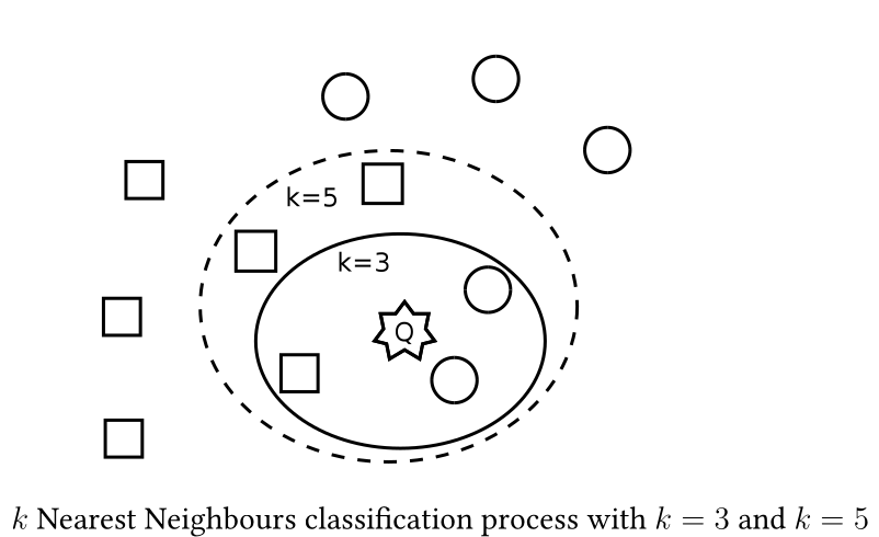
• k-NN Classifier
• Data Reduction Techniques
• Dealing with noise using large k
• Editing algorithms (for noise removal)
  • Edited Nearest Neighbor Rule
  • All k-NN
  • Multiedit
• Condensing algorithms (They select prototypes)
  • Condensing Nearest Neighbor Rule
  • IB2
• Data abstraction (generation) algorithms (They generate prototypes)
  • The algorithm of Chen and Jozwik
  • Reduction by Space Partitioning

k-NN Classifier

• Extensively used and effective lazy classifier
• Easy to be implemented
• It has many applications
• It works by searching the database for the k nearest items to the unclassified item
• The k nearest items determine the class where the new item belongs to
• The "closeness" is defined by a distance metric

Weaknesses of k-NN classifier

• High computational cost: k-NN classifier needs to compute all distances between an unclassified item and the training data
• High storage requirements: The training database must be always available
• Noise sensitive algorithm: Noise and mislabeled data, as well as outliers and overlaps between regions of classes affect classification accuracy

Example

Data

import matplotlib.pyplot as plt
from math import sqrt

points = [    
    [1,1,"Red"],
    [1,2,"Red"],
    [2,1,"Black"],
    [3,4,"Black"],
    [4,6,"Black"]
]

plt.title("Points")
plt.xlabel("x")
plt.ylabel("y")

for point in points:
    plt.plot(point[1],point[0], "o", color=point[2])

Function for euclidean distance

$d_{ij} = \sqrt{ \sum_{i=1}^{p} (X_{ik} - X_{jk})^2 }$

def euc_dis(point1, point2):
    return sqrt( (point1[0]-point2[0])**2 + (point1[1]-point2[1])**2 )

Function for k-NN Classification

def knn(point, points, k):
    result = 0;
    distance = []
    for i in range(len(points)):
        distance.append([euc_dis(point, points[i]), points[i][2]])
        distance.sort()
        
    for i in range(k):
        if distance[i][1] == "Red":
            result += 1
        else:
            result -= 1
            
    if result >= 0:
        return "Red"
    else:
        return "Black"   

Calling the k-NN function

print("The point [2,1] is:", knn([2,1], points, 3), " with K=3")
print("The point [2,1] is:", knn([2,1], points, 5), " with K=5")

The point [2,1] is: Red  with K=3
The point [2,1] is: Black  with K=5

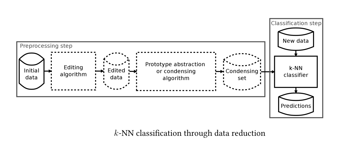
Data Reduction Techniques

Condensing and Prototype Abstraction (PA) algorithms

• They deal with the drawbacks of high computational cost and high storage requirements by building a small representative set (condensing set) of the training data
• Condensing algorithms select and PA algorithms generate prototypes
• The idea is to apply k-NN on this set attempting to achieve as high accuracy as when using the initial training data at much lower cost and storage requirements

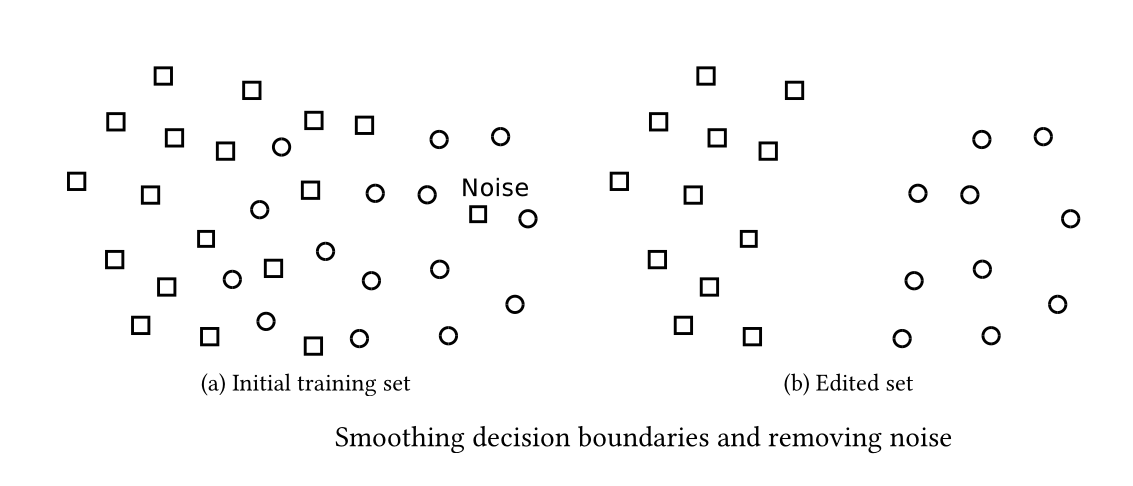
Editing algorithms

• They aim to improve accuracy rather than achieve high reduction rates
• They remove noisy and mislabeled items and smooth the decision boundaries. Ideally, they build an a set without overlaps between the classes
• The reduction rates of PA and condensing algorithms depend on the level of noise in the training data
• Editing has a double goal: accuracy improvement and effective application of PA and condensing algorithms

Dealing with noise using large k

• In general, the value of k that achieves the highest accuracy is dataset dependent
• Usually, larger k values are appropriate for datasets with noise since they examine larger neighborhoods
• However, large k values fail to clearly define the boundaries between distinct classes
• Determining the best k is a time consuming procedure
• Even the best k may not be optimal. Different k values may be optimal for different areas of the multidimensional space

Editing algorithms (for noise removal)

Edited Nearest Neighbor Rule (or Wilson's editing)

• The first editing algorithm and the basis of all other editing algorithms
• A training item is considered as noise and removed if its class label is different from the majority of its k nearest neighbours

Drawbacks

• It is parametric algorithm: k should be adjusted through time-consuming trial-end-error procedures
• High preprocessing cost: ENN-rule needs to compute: $\frac{N \cdot (N-1)}{2}$ distances

# ENN-rule

All k-NN

• Well-known variation of ENN-rule
• It iteratively executes ENN-rule with different k values
• In this way, it tries to remove even more noisy items

Drawbacks

• It is parametric algorithm: kmax should be adjusted through time-consuming trial-end-error procedures
• High preprocessing cost: All k-NN needs to compute: $\frac{N \cdot (N-1)}{2}$ distances

# All k-NN

Multiedit

• It is also based on ENN-rule
• Initially the training set is divided into n random subsets
• It applies ENN-rule (with k=1) over each item of each one subset, but searching for the nearest neighbour in the modn following subset
• The misclassified items are removed
• The whole process is repeated until the last R iterations produce no editing

Drawbacks

• It is parametric algorithm: n and R should be adjusted through time-consuming trial-end-error procedures
• It usually has even higher preprocessing cost than ENN-rule and All k-NN
• It may consider non-noisy items as noise. It may eliminate entire classes
• It is based on a random formation of subsets. Repeated applications may build a different edited set from the same training data

# Multiedit

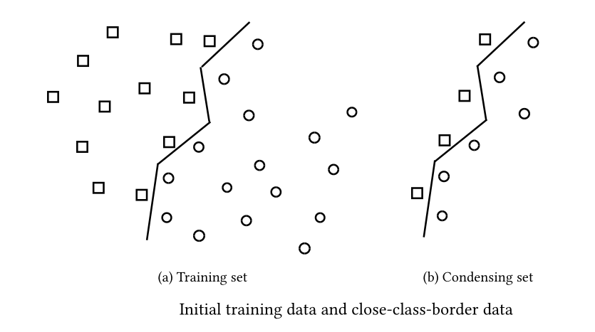
Condensing algorithms (They select prototypes)

Condensing Nearest Neighbor Rule

• CNN-rule is the earliest and a reference Condensing algorithm
• Items that lie in the “internal” data area of a class (i.e., far from class decision boundaries) are useless during the classification process. They can be removed without loss of accuracy
• CNN-rule tries to place into the condensing set only the items that lie in the close-class-border data areas
• CNN-rule tries to keep the close-class-border items as follows:
  • Initially, an item of the training set (TS) is moved to the condensing set (CS)
  • Then, CNN-rule applies 1-NN rule and classifies the items of TS by scanning the items of CS
  • If an item is misclassified, it is moved from TS to CS
  • The algorithm continues until there are no moves fromTS to CS during a complete pass of TS (This ensures that the content of TS is correctly classified by the content of CS)
  • The remaining content of TS is discarded
• The main idea behind CNN-rule is that if an item is misclassified, it is close to a border area and so it must be placed into the Condensing Set (CS)
• CNN-rule ensures that all removed TS items can be correctly classified by the content of CS

Advantages

• Non parametric

Drawbacks

• Order dependent
• Memory based
• Non incremental

# CNN-rule

IB2

• Is a fast one-pass version of CNN-rule
• Like CNN-rule:
  • Is non-parametric
  • Is order dependent
• Contrary to CNN-rule:
  • Does not ensure that all discarded items can be correctly classified by the CS
  • Builds its condensing set incrementally (appropriate for dynamic/streaming environments)
  • Does not require that all training data reside into the main memory
• Each training item x ∈ T S is classified using the 1-NN classifier on the current Condensing Set (CS)
• If x is classified correctly, it is discarded. Otherwise, x is transferred to CS

Note: New training data segments can update an existing condensing set in a simple manner and without considering the “old” (removed) data that had been used for the construction of CS

# IB2

Data abstraction (generation) algorithms (They generate prototypes)

The algorithm of Chen and Jozwik

• Chen and Jozwik’s algorithm (CJA) initially retrieves the most distant items, x and y in TS (diameter) and divides TS into two subsets: items that lie closer to x are placed in Sx whereas items that lie closer to y are placed in Sy
• CJA proceeds by selecting to divide subsets that contain items of more than one classes (non-homogeneous subsets). The non- homogeneous subset with the largest diameter is divided first. If all subsets are homogeneous, CJA continues by dividing the homogeneous subsets
• This procedure continues until the number of subsets becomes equal to a user specified value
• For each created subset S, CJA averages the items in S and creates a mean item that is assigned the label of the majority class in S. The mean items created constitute the final condensing set.
• CJA selects the next subset that will be divided by examining its diameter. The idea is that a subset with a large diameter probably contains more training items. Therefore, if this subset is divided first, a higher reduction rate will be achieved.

CJA properties:

• It builds the same CS regardless of the ordering of the data in TS
• It is parametric
• The items that do not belong to the most common class of the subset are not represented in CS

# CJA

Reduction by Space Partitioning

• CJA is the ancestor of RSP algorithms
• RSP1 computes as many mean items as the number of different classes in each subset (it does not ignore items)
• RSP1 builds larger CS than CJA
• It attempts to improve accuracy since it takes into account all training items
• Similar to CJA, RSP1 uses the subset diameter as the splitting criterion, based on the idea that the subset with the larger diameter may contains more training items, and so, a higher reduction rate could be achieved.
• RSP1 and RSP2 differ on how they select the next subset to be divided
• RSP2 uses as its splitting criterion the highest overlapping degree
• The overlapping degree of a subset is the ratio of the average distance between items belonging to different classes and the average distance between items that belong to the same class.
• RSP3 continues splitting the non-homogeneous sub-sets and terminates when all of them become homogeneous
• It can use either the largest diameter or the highest overlapping degree as spiting criterion
• RSP3 is the only RSP algorithm (CJA included) that automatically determines the size of CS
• like CJA, RSP1 and RSP2, CS built by RSP3 does not depend on the data order in TS

# RSP3

• The algorithm:

  • It utilizes a simple data structure S to hold the unprocessed subsets
  • Initially, the whole TS is an unprocessed subset
  • At each repeat-until iteration, RSP3 selects the subset C with the highest splitting criterion value
  • If C is homogeneous, the mean item is computed by averaging the items in C and is paced in CS
  • Otherwise, like CJA, C is divided into two subsets D1 and D2
  • These new subsets are added to S
  • The repeat-until loop continues until all subsets are homogeneous

• RSP3 properties:

  • It generates few prototypes for representing non close class-border areas, and many prototypes for representing close-class-border areas
  • The reduction rate achieved by RSP3 highly depends on the level of noise in the data
  • Finding the most distant items in each subset implies the computations of all distances between the items of the subset